ai/gradient-descent-how-a-computer-learns-a-number-by-rolling-downhill.md
Gradient descent: how a computer learns a number by rolling downhill
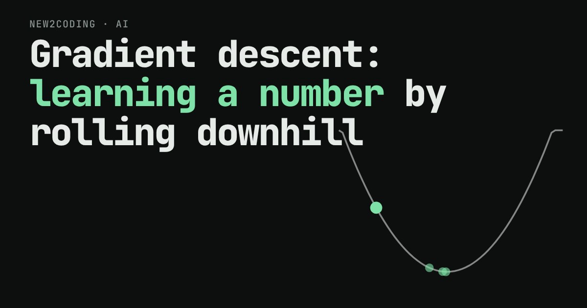
How does a computer learn a number? It can't solve for it in one go. It tries a guess, measures how wrong it is, and nudges the guess downhill.
This article shrinks that idea to one weight and four data points. You drag a ball along a loss curve, take steps, and change the learning rate to see why too small is slow and too big makes things worse. You also get a six-line Python loop with real output, and a short note on how the same loop trains models with billions of weights.
Imagine a program that has to learn one number. You give it four examples, and it has to find the number that fits them best. It can't solve a formula in its head. All it can do is try a number, measure how wrong it is, and adjust. That loop is how nearly every modern AI model is trained, and it has a name: gradient descent.
The smallest possible model
Suppose you track how many hours you study (x) and the score you get on a short quiz (y):
| hours (x) | 1 | 2 | 3 | 4 |
|---|---|---|---|---|
| score (y) | 2 | 4 | 5 | 8 |
Our model is a single rule: prediction = w × x. The number w is called a weight: it is the thing the model learns. If w = 2, the model predicts 2, 4, 6 and 8, which is close but not exact. Which w is best?
Measuring "how wrong"
To improve, the program needs a single number that says how bad the current guess is. This is called the loss. A common choice: for each example take the error (prediction minus real answer), square it so that negative and positive errors don't cancel out, then average them. This is the mean squared error.
For w = 0 the model predicts 0 for everything, and the loss is 27.25. For w = 1.9 the loss is 0.175, the lowest it can go for this data. Plot the loss for every possible w and you get a smooth bowl-shaped curve. Training means finding the bottom of the bowl.
Which way is downhill?
The program can't see the whole bowl. It only knows the loss at its current w, plus one more thing: the gradient, which is the slope of the curve at that point. (With one weight, the gradient is just an ordinary slope. With many weights it is one slope per weight.)
- If the slope is negative, the curve is going down to the right, so increase
w. - If the slope is positive, the curve is going down to the left, so decrease
w. - If the slope is near zero, you are near the bottom, so stop moving.
That gives one rule: w = w − learning_rate × slope. The learning rate decides how big a step to take. For our data the slope works out to 15 × w − 28.5 (you can get this with a little calculus, or just trust the code below, which computes it directly).
Try it: roll the ball downhill
With a learning rate of 0.05 the ball slides to the bottom in a handful of steps, and the steps shrink on their own, because the slope shrinks as the curve flattens. With 0.01 it gets there too, only slowly. With 0.1 it overshoots the bottom and zigzags across it before settling. With 0.14, each overshoot is bigger than the last, and the loss grows instead of shrinking. (For this particular curve the tipping point is about 0.133; a different problem has a different limit.)
The same loop in code
xs = [1, 2, 3, 4]
ys = [2, 4, 5, 8]

def loss(w):
    return sum((w * x - y) ** 2 for x, y in zip(xs, ys)) / len(xs)

def slope(w):
    return sum(2 * (w * x - y) * x for x, y in zip(xs, ys)) / len(xs)

w = 0.0
learning_rate = 0.05
for step in range(1, 6):
    w = w - learning_rate * slope(w)
    print(step, round(w, 3), round(loss(w), 3))
Running it prints:
1 1.425 1.867
2 1.781 0.281
3 1.87 0.182
4 1.893 0.175
5 1.898 0.175
Five steps took the loss from 27.25 to about 0.175. Nobody told the program the answer. It only ever looked at its current error and the slope.
From one weight to billions
Real models have far more than one weight: a large language model can have billions of them. The loop is the same. Compute how wrong the model is on some training examples, find the slope for every weight (the method that does this efficiently in neural networks is called backpropagation), nudge each weight a little in its downhill direction, and repeat. Two practical differences are worth knowing: the loss "bowl" has many dimensions and is rarely a perfect smooth bowl, and instead of using all the data for every step, training usually uses a small random batch each time (a variant called stochastic gradient descent), which is cheaper per step.
What to take away
When you read "the model was trained", picture this loop running an enormous number of times: measure the error, find the downhill direction, take a small step. The learning rate is one of the settings people tune by hand, and as the demo shows, too small wastes time while too big can make things worse. Next time a training run "doesn't converge", this is the first thing to suspect.